PMI for images (scratch)

Posted: 2016-08-01 , Modified: 2016-09-05

Results

PMI distribution

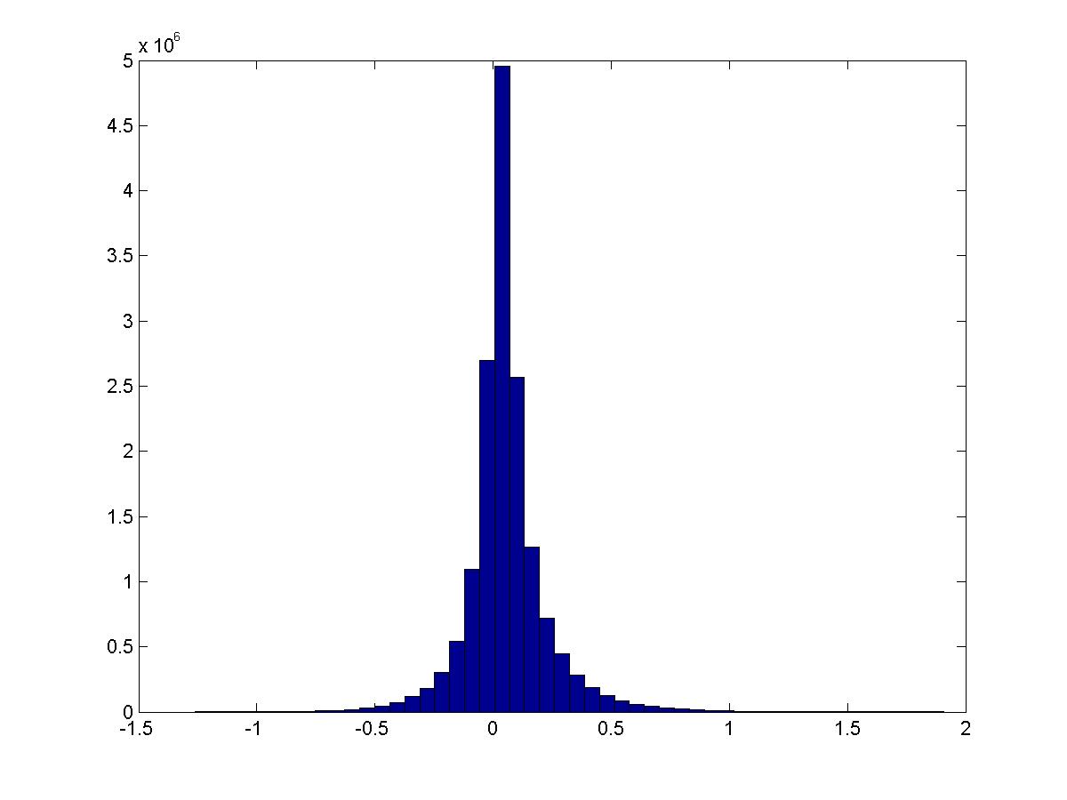
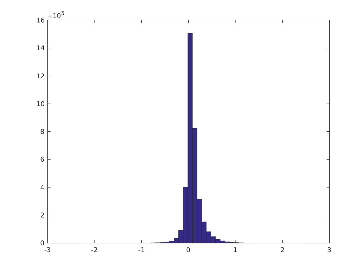
Over all pairs of features \(i,j\), this is the distribution of \(PMI(v_i,v_j)\):

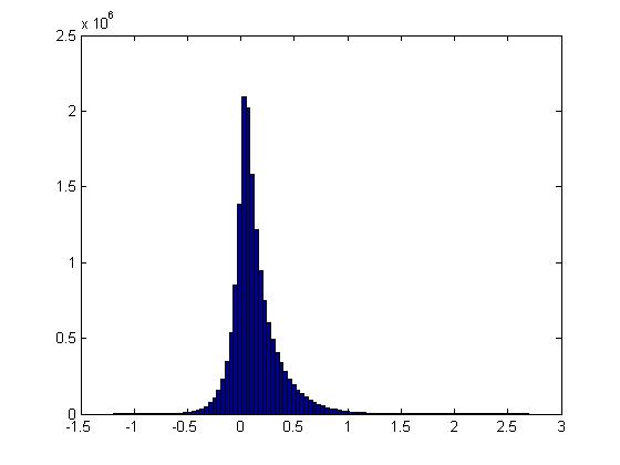
(Question: is this what you would expect if the distribution were “random” or are the tails different than what we would expect?)

Is there a correlation between PMI and distance between features? (Distance ranges from \(0\) to \(5\sqrt 2\).) It seems not.

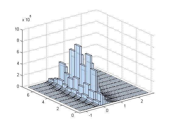
Conditioned on the digit being a specific value, how does the PMI distribution look? Still about the same… except that 1 has much larger activation. These are digits 0-4.

Thresholded PMI distribution

See script pmi_thresholded.m.

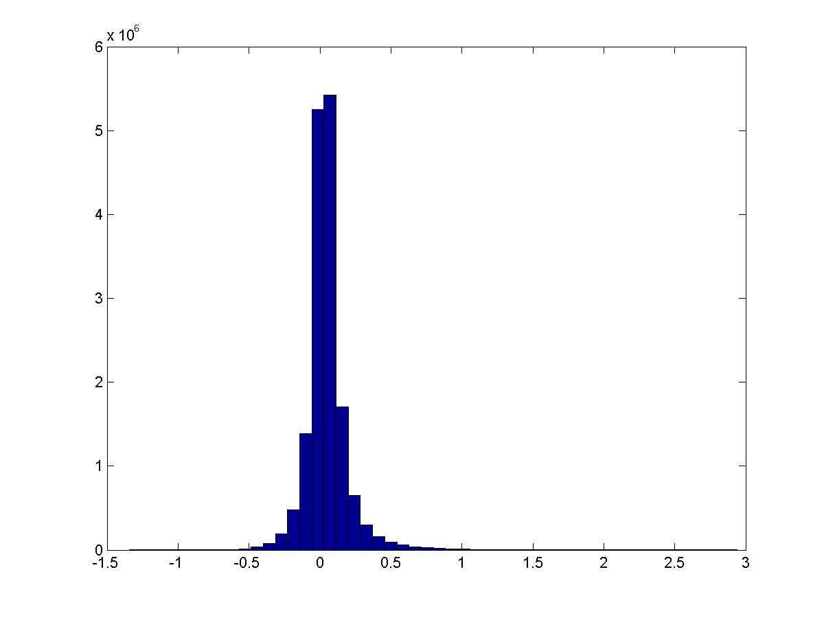
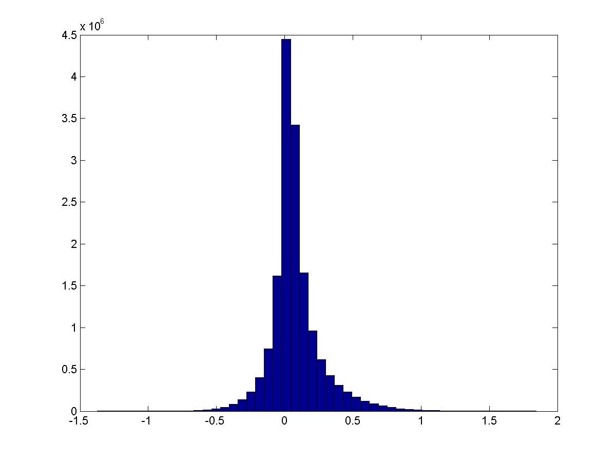
Remove all features that do not have PMI \(>1\) with another feature. Now do the same thing.

This is the distribution of \(PMI(v_i,v_j)\):

These are digits 0-4.

Percentiles of the distributions (\(i\)th row is 0, 10, 20, … 100% for the CPMI’s of digit \(i\), last row is PMI over all digits).

  Columns 1 through 7

   -0.9746   -0.0588   -0.0140    0.0112    0.0306    0.0488    0.0681
   -3.1365   -0.3102   -0.0940    0.0050    0.0609    0.1144    0.1812
   -0.9300   -0.0626   -0.0130    0.0134    0.0333    0.0526    0.0740
   -0.7660   -0.0462   -0.0022    0.0210    0.0403    0.0602    0.0835
   -2.0740   -0.0565   -0.0071    0.0188    0.0397    0.0611    0.0855
   -0.8674   -0.0628   -0.0077    0.0229    0.0471    0.0705    0.0966
   -2.3770   -0.0457   -0.0007    0.0228    0.0428    0.0639    0.0886
   -2.4824   -0.0928   -0.0235    0.0121    0.0379    0.0633    0.0925
   -0.9435   -0.0521   -0.0066    0.0161    0.0347    0.0545    0.0785
   -2.1549   -0.0505   -0.0020    0.0231    0.0446    0.0679    0.0961
   -0.8693   -0.0515    0.0008    0.0344    0.0640    0.0949    0.1309

  Columns 8 through 11

    0.0910    0.1215    0.1730    1.5181
    0.2772    0.4314    0.7470    5.3609
    0.1007    0.1393    0.2117    1.5297
    0.1141    0.1604    0.2521    1.6011
    0.1169    0.1635    0.2537    2.2486
    0.1293    0.1773    0.2773    2.0363
    0.1215    0.1727    0.2771    2.5443
    0.1305    0.1882    0.3019    2.9006
    0.1111    0.1639    0.2788    2.1102
    0.1344    0.1957    0.3210    2.7701
    0.1761    0.2406    0.3557    1.7908

Thresholded PMI distribution

See script pmi_thresholded.m.

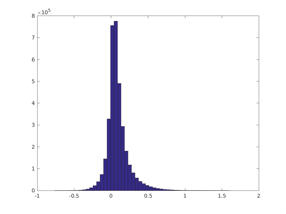
Remove all features that do not have PMI \(>1\) with another feature. Now do the same thing.

This is the distribution of \(PMI(v_i,v_j)\):

These are digits 0-4.

Thresholded PMI distribution

Thresholding by psiTr

CODE: Run pmi_thresholded and check_top_pmis.

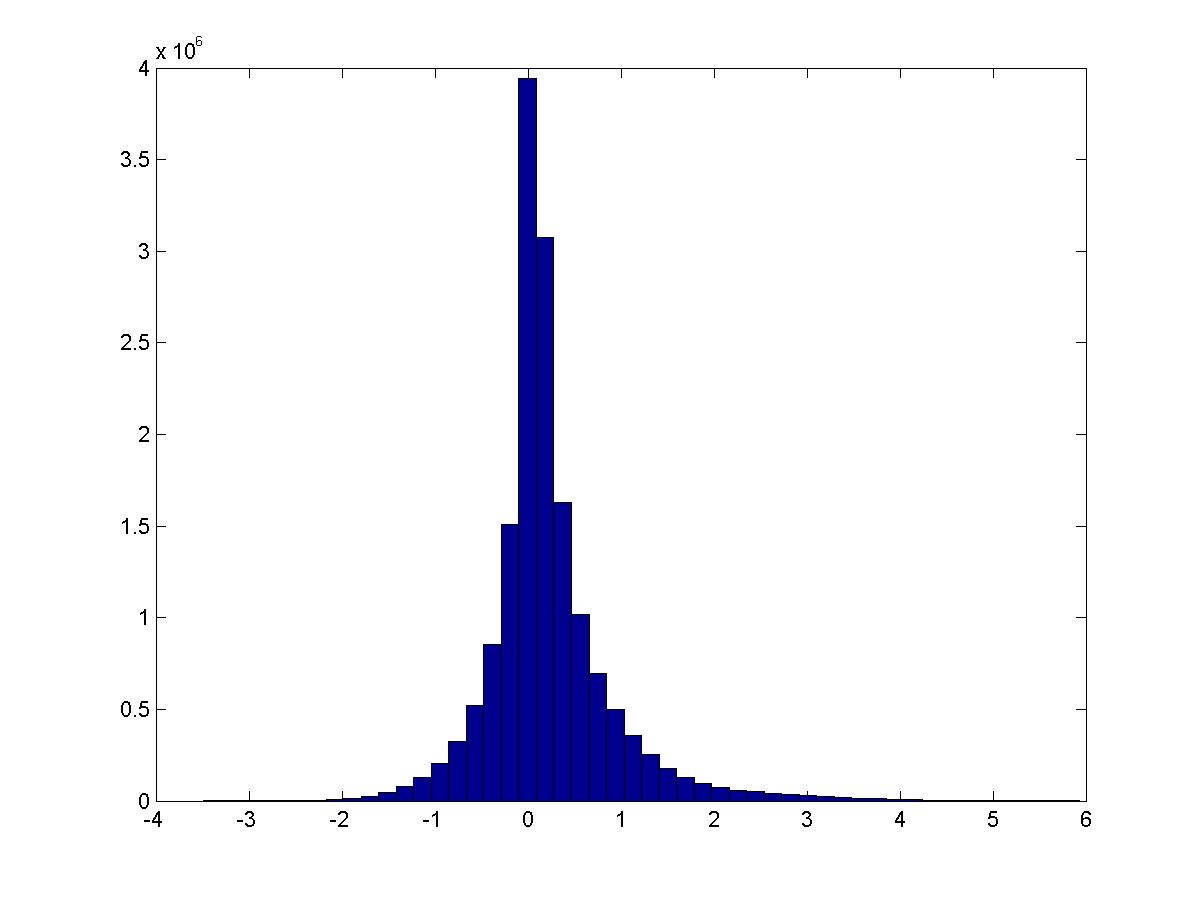
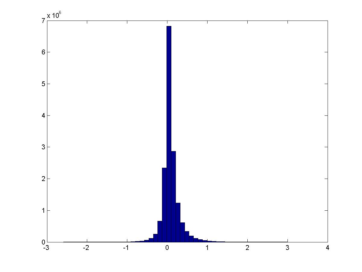
Remove all features that do not have activation \(>1\) in some image. Now do the same thing. (NOTE: the maximum PMI is less because the max PMI’s are between features that have small activation. Try this again thresholding by PMI?)

This is the distribution of \(PMI(v_i,v_j)\):

These are digits 0-9.

Percentiles of the distributions (\(i\)th row is 0, 10, 20, … 100% for the CPMI’s of digit \(i\), last row is PMI over all digits). (Note the last column is different)

  Columns 1 through 7

   -0.9746   -0.0588   -0.0140    0.0112    0.0306    0.0488    0.0681
   -3.1365   -0.3102   -0.0940    0.0050    0.0609    0.1144    0.1812
   -0.9300   -0.0626   -0.0130    0.0134    0.0333    0.0526    0.0740
   -0.7660   -0.0462   -0.0022    0.0210    0.0403    0.0602    0.0835
   -2.0740   -0.0565   -0.0071    0.0188    0.0397    0.0611    0.0855
   -0.8674   -0.0628   -0.0077    0.0229    0.0471    0.0705    0.0966
   -2.3770   -0.0457   -0.0007    0.0228    0.0428    0.0639    0.0886
   -2.4824   -0.0928   -0.0235    0.0121    0.0379    0.0633    0.0925
   -0.9435   -0.0521   -0.0066    0.0161    0.0347    0.0545    0.0785
   -2.1549   -0.0505   -0.0020    0.0231    0.0446    0.0679    0.0961
   -0.8693   -0.0515    0.0008    0.0344    0.0640    0.0949    0.1309

  Columns 8 through 11

    0.0910    0.1215    0.1730    1.5181
    0.2772    0.4314    0.7470    5.3609
    0.1007    0.1393    0.2117    1.5297
    0.1141    0.1604    0.2521    1.6011
    0.1169    0.1635    0.2537    2.2486
    0.1293    0.1773    0.2773    2.0363
    0.1215    0.1727    0.2771    2.5443
    0.1305    0.1882    0.3019    2.9006
    0.1111    0.1639    0.2788    2.1102
    0.1344    0.1957    0.3210    2.7701
    0.1761    0.2406    0.3557    1.7908

TODO: add data from check_top_pmis. This produces a graph showing which features are close to each other.

SVD-SVM

Run qsub svd_svm.cmd which runs svd_testing2.m, or sbatch slurm_svd.cmd. The results are saved in accs_1.mat.

Results:

Dimension	Last	Best
500	99.26	99.44
100	97.5	98.82
50	96.84	96.84

Weighted SVD-SVM

Do weighted SVD (as in the NLP paper) and then train a SVM. Note this does worse than just SVD! Why?

Dimension	Last	Best
50	95.44	96.8

PMI suitability

Is PMI the right measure? Are the feature vectors close to sparse? if the average image there is \(>20\%\) activation, then no.

For the first 10 images, this is what the percentiles look like:

percentiles:

pcs =

   100    99    95    90    80    70

Image 1 (label 5)
    2.3230
    1.2966
    0.8840
    0.6766
    0.4381
    0.3140

Image 2 (label 0)
    2.1275
    1.3604
    0.9482
    0.7418
    0.5036
    0.3769

Image 3 (label 4)
    1.7975
    0.9874
    0.6185
    0.4704
    0.3145
    0.2247

Image 4 (label 1)
    2.2506
    1.2399
    0.7160
    0.4949
    0.3029
    0.1992

Image 5 (label 9)
    2.0837
    1.3970
    0.8726
    0.6461
    0.3937
    0.2707

Image 6 (label 2)
    2.4831
    1.4978
    1.0466
    0.7880
    0.5002
    0.3544

Image 7 (label 1)
    2.5064
    1.3688
    0.7591
    0.5203
    0.3089
    0.1935

Image 8 (label 3)
    3.3030
    1.6943
    1.1588
    0.8658
    0.5756
    0.4070

Image 9 (label 1)
    2.2263
    0.9396
    0.4905
    0.3279
    0.1944
    0.1178

Image 10 (label 4)
    2.2420
    1.3486
    0.8494
    0.6169
    0.3751
    0.2586

This looks pretty good—the top 1% of features are much larger than the rest.

Look for discriminative features, those that occur with one label and rarely for others. (I arbitrarily define this as: the maximum average activation is \(>1.5\) times the second largest, and the maximum is at least 0.1. I exclude the digit 1 (indexed as 2).)

sig_act_inds = intersect(find(m1>=1.5*m2), find(m1>0.1));
sig_act_inds2 = intersect(sig_act_inds, find(am1 ~=2));

115/7200 features fit this criterion.

Do SVM coefficients have negative weights?

PMI and geometry

collect, same patch; no collect, same patch; horiz collect; horiz no collect; vert collect; vert no collect; all

ans =

  Columns 1 through 7

   -0.9605   -0.3457   -0.2067   -0.1000   -0.0103    0.0783    0.1698
   -1.0872   -0.0690   -0.0062    0.0281    0.0563    0.0880    0.1277
   -1.5676   -0.3858   -0.2386   -0.1310   -0.0454    0.0409    0.1303
   -0.9235   -0.0241    0.0307    0.0621    0.0919    0.1266    0.1695
   -1.3763   -0.3810   -0.2237   -0.1053   -0.0072    0.0839    0.1708
   -0.9163   -0.0108    0.0284    0.0530    0.0796    0.1093    0.1458
   -1.1984   -0.0727   -0.0094    0.0253    0.0534    0.0847    0.1241

  Columns 8 through 11

    0.2735    0.3922    0.5678    1.3093
    0.1821    0.2624    0.4080    2.4518
    0.2220    0.3257    0.4557    1.1007
    0.2240    0.3054    0.4534    2.6332
    0.2607    0.3593    0.4863    0.9118
    0.1942    0.2660    0.3970    2.6332
    0.1778    0.2587    0.4034    2.6897

Unorganized

I sorted pairs of features by PMI value and took the largest 10000 pairs. The majority of the pairs (~77%) have strongest activation with the digit 1. (The digit 1 has conditional PMI values that are much larger than all the other digits - don’t know what to do about this.) 85% of the pairs have highest activations with the same digit.

If the pair has strong activation with 1, then it’s often much larger than the other activations.

Otherwise this is not necessarily true. A typical non-1 feature has average activations with the 10 digits that looks something like this:

  Columns 1 through 7

    0.0708    0.2673    0.0940    0.1537    0.2122    0.1116    0.2627

  Columns 8 through 10

    0.2947    0.1448    0.3361

Notes

Experiments:

mnist_testing.m: Prep data.
svd_testing.m: How does reducing the number of features through SVD affect classification accuracy?
pairwise_mi.m: Tests related to mutual information
mi.m
MI_GG.m
rsvd.m

	         nlayers: 2
             layer: {2x1 cell}
    type_zerolayer: 2
             ndesc: 7200


                         numlayer: 1
                        centering: 0
    median_contrast_normalization: 0
                           npatch: 5
                      subsampling: 2
                             smap: 50
                   type_zerolayer: 2
                            sigma: 0.7459
                                Z: [25x50 double]
                                w: [50x1 double]

In pairwise_mi.m there’s no normalization by scaling (\(-2\log\pat{scale}\)).

https://en.wikipedia.org/wiki/Conditional_mutual_information

Theory

The right PMI measure to use here is \[ \ln \pf{\an{v,w}}{\an{v,\one}\an{w,\one}}. \] Because if we assume the activations are like \((e^{\chi,v})_\chi\), then we still get that the expected dot product of these is \(\int e^{\an{\chi,v}}e^{\an{\chi,w}}\,d\chi\propto \exp\pa{\fc{\ve{v+w}^2}{2}}\).

Thoughts

Is a picture more like a context or a document? We’re treating it like context (looking at all pairs of features there). But its size makes it seem more like a document. Or better: a sentence, because sentences are big enough to incorporate different features and small enough to still have a vector associated with it.
How to incorporate convolutional ideas? Ex. if features \(f_1,f_2\) are in the same relationship (translationally) as \(f_1',f_2'\) then we expect PMI to be similar, so we should we really be looking at a \(7200\times 7200\) matrix? How about look at PMI of adjacent features? (But they shouldn’t overlap…) Or look at PMI pre-convolution by another layer?
What happens if you apply (convolutional?) DL to the learned features? Then apply SVD to the dimension-reduced vectors?

Todo

Coding

Completed
Compute PMI matrix.
Plot histogram of PMI’s.
Plot histogram of conditional PMI’s. (They don’t look like they have higher values… Try thresholding first? Look at features with largest PMI? Calculate entropies?)
Look at correlations between PMI’s and distances between pairs. (There doesn’t seem to be any correlation.)
Train on feature vectors.
Do weighted SVD on PMI matrix.
Todo:
Do dictionary learning on feature vectors/PMI vectors (?).
Do unsupervised learning: k-means on feature vectors and on original (baseline).
Try clustering based on graph diffusion with PMI’s giving distances.
Try taking SVD of features for each patch first (ex. reduce from 200 to 10; this gives 360-dimensional). How does this compare to SVD after of everything taken together? (Probably worse.)
Do SVD/weighted SVD of each patch only comparing with neighboring patches.
Geometry

(Compare to purely random.)

Theory

Understand loss function for PMI.

Scratch

Why is the normalization nrm=mean(sqrt(sum(compTr.^2)))?

Steps, Experiments

Run experiments.

nohup nice -19 matlab -nodisplay -nodesktop -nojvm -nosplash < run_experiments2.m > output_2016-08-07.txt 2>&1 &

%Get psiTr
pmi_experiments('logs/model_mnist_5_2_0_2_2_0_50_200_0_1.000000e-01_1.000000e-01_1.000000e-01_2.mat');
%get percentiles for each feature
pc= get_percentiles(psiTr);
save('pc_1.mat','pc','-v7.3');
%calculate PMI after normalizing and deleting zero rows.
[P, inds] = calculate_pmi(psiTr); %inds give the indices that are kept (indices of nonzero rows)
%exploratory analysis
%pmi_experiments(P);
[all_pmi_pairs, positions, dists] = pmi_experiments2(P, inds');
save('all_pmi_pairs_1.mat','all_pmi_pairs');
save('positions_1.mat','positions');
save('dists_1.mat','dists');

%cpmi matrices
Ps = calculate_cpmi(psiTr, Ytr, '1');
cpmi_experiments('P_1');

Guide to data

psiTr_1.mat, psiTe_1.mat etc. are the feature vectors for the training/test sets and the different architectures. The architectures are
1. test_ckn([5 2 0],[2 2 0],[50 200 0],2,'mnist'); (7200, 0.57%)
2. test_ckn([1 3 0],[2 2 0],[12 50 0],3,'mnist'); (1800, 0.63%)
3. test_ckn([1 3 0],[2 4 0],[12 400 0],3,'mnist'); (3600, 0.41%)