(BKS15) Dictionary Learning and Tensor Decomposition via the Sum-of-Squares Method

Theorem. Given \(\ep>0,\si\ge 1, \de>0\) there exists \(d\) and a polytime algorithm that given input

• a \(\si\)-dictionary \(n\times m\),
• \((d,\tau=n^{-\de})\)-nice \(\{x\}\),
• \(n^{O(1)}\) samples from \(y=Ax\),

outputs with probability \(\ge 0.9\) a set \(\ep\)-close to columns of \(A\).

• A \(\si\)-dictionary has \(AA^T\preceq \si I\) (analytic proxy for overcompleteness \(\fc mn\)).
• A distribution is \((d,\tau)\)-nice if \(\E x_i^{d/2}x_j^{d/2}\le \tau\) for all \(i\ne j\), and \(\E x^\al=0\) for all \(|\al|\le d\). (Ex. Bernoulli(\(\tau\)) times Gaussian with \(\E z_i^d = \rc\tau\).)

Note on running time:

• \(\ep\)-accuracy with running time depending on \(\poly\prc{\ep}\) in the exponent. So this is better for giving an initial solution for local search methods.

Noisy tensor decomposition 1

Given noisy version of \(\sumo im \an{a^i, u}^d = \ve{A^Tu}_d^d\), recover \(\{a^1,\ldots, a^m\}\).

Theorem (Noisy tensor decomposition). For every \(\ep>0,\si\ge 1\) there exist \(d,\tau\) such that a probabilistic \(n^{O(\ln n)}\)-time agorithm, given \(P\) with \[\ve{A^T u}_d^d - \tau \ve{u}_2^d \preceq P \preceq \ve{A^Tu}_d^d + \tau \ve{u}_2^d,\] outputs with probability 0.9 \(S\) that is \(\ep\)-close to \(\{a^1,\ldots, a^m\}\). (\(\preceq\) means the difference is a sum of squares.)

Note this allows significant noise since we expect \(\ve{A^Tu}_d^d\sim mn^{-\fc d2}\ll \tau\).

Reduction

Take \[ P = \EE_{i} \an{y_i, u}^{2d}.\]

Algorithm

1. Use SoS to find degree-\(k\) pseudo-distribution \(\{u\}\) that maximizes \(P(u)\) under \(\ve{u}^2=1\).
2. Let \(W\) be a product of \(O(\ln n)\) rndom linear functions.
3. Output top eigenvector of \(M\), \(M_{ij} = \wt \E W(u)^2 u_iu_j\).

SoS Algorithm: given \(\ep>0, k,n,M\), \(P_1,\ldots, P_m\in \R[x_1,\ldots, x_n]\) with coefficients in \([0,M]\), if there exists a degree \(k\) pseudo-distribution with \(P_i=0,i\in [m]\), then we can find \(u'\) satisfying \(P_i\le \ep, P_i\ge -\ep\) for every \(i\in [m]\) in time \((n\polylog\prc{M}{\ep})^{O(k)}\).

(Proof: This is a feasibility problem. Use ellipsoid method.)

Steps

1. If \(u\) is an actual distribution, the the output is close to a column.
2. Generalize to pseudo-distributions.
3. Generalize to getting all columns.

Idea: If not correlated, then \(P(u)\) is small. The inequalities can be turned into polynomial inequalities provable by SoS.

Noisy tensor decomposition

Theorem (Noisy tensor decomposition, 4.3). There is a probabilistic algorithm that given

• \(\ep>0\)
• \(\si \ge 1\)
• degree \(d\ge d(\ep,\si) = O\pf{\ln \si}{\ep}\)
• noise parameter \(\tau \le \tau(\ep) = \Om(\ep)\)
• degree \(d\) polynomial \(P\in \R[u]\) such that \[\ve{A^T u}_d^d - \tau \ve{u}_2^d \preceq P \preceq \ve{A^Tu}_d^d + \tau \ve{u}_2^d,\] outputs with high probability \(S\) that is \(\ep\)-close to \(\{a^1,\ldots, a^m\}\). (\(\preceq\) means the difference is a sum of squares.)

Algorithm

1. Start with \(S=\phi\). Let \(\ga = \fc{C}{\ep}\) for \(C\) large enough. ?? What’s \(k\)?
2. Loop:
   1. Attempt to find a degree \(k\) pseudo-distribution \(U\) satisfying the constraints \(P(U) \ge 1-\tau\), \(\ve{U}_2^2=1\), \(\an{s,U}^2\le 1-\ga\) for every \(s\in S\) (to repel it away from vectors we already found). If fail, stop.
   2. Use the “sampling pseudo-distributions” algorithm to obtain a unit vector \(c'\) such that \[\begin{align} P(c') & \ge e^{-\ep d} - \tau\\ \ep &:= O(\pf{\tau}{d} + \fc{\ln \si}{d} \fc{\ln m}k) \end{align}\]
   3. Add \(c'\) to \(S\).

Sampling pseudo-distributions

Proof

1. Existence of \(c'\).
   • \(U\) exists because any column of \(A\) is a solution. (CHECK columns far!!)
   • \(U\) is correlated with \(A\): By assumption, for \(\ve{U}_2^2=1\), \(P\in \ve{A^T U}_d^d + \tau[-1,1]\). Thus \(P(U)\ge 1-\tau\) implies \[\ve{A^TU}_d^d \ge 1-2\tau.\]

   • If \(U\) correlates well with \(A\), then \(U\) correlates with some column of \(A\).

     Lemma 6.1. Given

     • \(A\) is \(\si\)-overcomplete
     • \(u\) is degree \(3k\) pd over \(\R^n\) satisfying \(\ve{A^Tu}_d^d \ge e^{-\de d}, \ve{u}_2^2 = 1\),
     • \(d-2\mid k\) (?? this seems to be necessary. Think of \(k\gg d\).)

     there exists a column of \(A\) such that \(\wt \E \an{c,u}^k \ge e^{-\ep k}\), \(\ep=O(\de + \fc{\ln \si}{d} + \fc{\ln m}k)\).

     • Motivation for proof: First, let’s see how to prove this if \(u\) is an actual vector. By averaging, there is a column such that \[ \ve{A_{\cdot i}^T u}_{k}^k \ge \pf{1-\ep}{m}\implies A_{\cdot i}^Tu \ge \pf{1-\ep}{m}^{\rc k}\approx e^{\fc{\ln m}{k}}.\] (This also shows why we expect \(\ln m\) in the exponent.) This averaging argument still works for pseudo-distributions when \(d=k\)—the first inequality still holds true, if we have \(d=k\). (The first inequality would no longer imply the second, though.) (?? Why wouldn’t we take \(d=k\)?)
     • ?? For some reason, we want to use an inequality not depending on \(m\) (depending on \(\ve{A^Tu}_2\) is good, because we have control of this using \(\si\)), in which case instead of using the inequality \(\ve{v}_{\iy} \ge \fc{\ve{v}_d}{m^{\rc d}}\) we use \(\ve{v}_{\iy}^{d-2}\ge \fc{\ve{v}_d^d}{\ve{v}_2^2}\). We need to change this into a SoS inequality, so replace \(\iy\) by \(k\) for \(k\) large, \[\ve{v}_d^{\fc{dk}{d-2}} \le \ve{v}_k^k (\ve{v}_2^2)^{\fc{k}{d-2}}\] provable by SoS (expand and then use Muirhead/AM-GM).
     • Proof. \[ \ve{A^Tu}_k^k \ge \fc{(\ve{A^Tu}_d^d)^{\fc k{d-2}}}{(\ve{A^Tu}_2^2)^{\fc{k}{d-2}}} \ge \fc{e^{-\de d}}{\si^{\fc k{d-2}}}. \] Now use averaging on \(\ve{A^Tu}_k^k\).
   • Here \(\de = O\pf{\tau}d\) so we get \[ \wt E \an{c,u}^k \ge e^{-\ep' k},\quad \ep' = O(\fc{\tau}d + \fc{\ln \si}{d} +\fc{\ln m}{k}).\] This means we set \(k=\boxed{\frac{C\ln m}{\ep}}\). This also means we need \(d=\Om(\rc{\ep}\ln \si)\), \(\tau=O(\ep)\).
   • Example: if \(u\) is the actual distribution \(u=A_{\cdot i}\) with probability \(\rc{m}\), then \(\wt E\an{c,u}^k = \rc m\). Hence we can’t do better than \(k=\Om(\ln m)\).

2. Now we analyze the algorithm to “sample pseudo-distributions”: given a PD that correlates with a vector, find a vector close to it. We prove:

   Theorem 5.1. The “sample pseudo-distributions” algorithm, given

   • even \(k\ge 0\)
   • degree \(k\) p.d. with \(\ve{u}_2^2=1\) and \(\wt \E\an{c,u}^k \ge e^{-\ep k}\) (?? I think we want this for \(k-2\).)

   outputs \(c'\in \R^n\) with \(\an{c,c'}\ge 1-O(\ep)\) with probability \(2^{-\fc{k}{\poly(\ep)}}\).

   • Here is the idea. We want to compute the tensor decomposition by using SVD (because there aren’t other good ways to compute overcomplete tensor decomposition…). Suppose that \(u\) were an actual distribution; since it is correlated with \(A\), it is approximately supported on columns of \(A\). Then \(\wt \E uu^T = \sum p_i a_i a_i^T\). The \(a_i\) are not uniquely identifiable from this (that’s the whole problem with SVD, why we want tensors in the first place!). Idea: consider \(\wt \E p(u) uu^T = \sum p_i p(a_i) a_ia_i^T\) instead. If \(p\) is a function that is large on \(a_i\) and small on all other \(a_j\), then we win. Take \(p\) to be a product of linear factors. If we put in enough factors, then with good probability the \(p(a_i)\) will become farther apart, and one outruns the others, \(|p(a_i)|\gg \sqrt m|p(a_i)|\). Take \(p =W^2\) where \(W\) is a product of \(O(\ln n)\) random linear functions \(\an{u,v}, \ve{v}_2=1\).

   • We are given \(c\) such that \(\wt E\an{c,u}^k \ge e^{-\de d}\) (high correlation) and we want that \(c\) to be a value of \(v\) that makes (the quadratic form) \(v\mapsto \wt \E W(U) \an{v,U}^2\) large. In fact, what we want is that when normalized so the sum of the eigenvalues is 1, the singular value corresponding to \(c\) is close to 1.

     There are 3 parts. (a) We need to understand how “renormalization” of pseudo-distributions works. (b) We need to show that for our choice of \(W\), we have with some probability a lower bound for \(\wt \E W(U) \an{c,U}^2\). This is the hardest part. (c) We need to show that \(c\) is close to the singular vector (which we output). (I think (c) is in essence a matrix/eigenvector perturbation result, but it’s cloaked in the language of SoS here—unravel!)
   • Lemma (reweighting). Let \(U\) be a degree \(k\) p.d. Then for every SoS polynomial \(W\) of degree \(d<k\), \(\wt \E W>0\), there exists a degree \((k-d)\) p.d. \(U'\) such that for every \(\deg P \le k-d\), \[\wt E_{U'} P(U') = \rc{\wt \E_U W(U)} \wt \E_{U} W(U)P(U).\] Proof. Just verify the positivity property.

   • Lemma 5.2. Let \(U\) be a degree-\(k+2\) pseudo-distribution over \(\R^n\) with \(\ve{U}_2^2=1\) and such that there exists a unit vector \(c\in \R^n\) such that \(\wt \E\an{c,u}^k \ge e^{-\ep k}\). \(W=\rc{M^{k/2}} \prod_{i=1}^{k/2} w^{(i)}\) where \(w^{(i)}\) are iid draws from \(w=\an{\xi,u}^2\), \(\xi\sim N(0,I_n)\). Then with probability \(2^{-O\pf{k}{\poly(\ep)}}\), \(\wt \E\an{c,u}^2W \ge (1-O(\ep))\wt \E W\).

     (?? Discrepancy between \(k\) and \(k+2\).)
   • By reweighting, there exists a degree 2 p.d. \(U'\) such that \[\wt \E_{U'} \an{v,u'}^2 = \rc{\wt \E_U W(U)} \wt\E_{U} W(U) \an{v,U}^2.\] By Lemma 5.2, the value at \(c\) is \(\ge 1-O(\ep)\).
   • Proof (Sketch). This is more likely to be true if \(\an{c,\xi}\) is large. Let \(w=\an{\xi,u}^2\). Let \(\tau_M\) be such that \(\E_{\xi_0|\xi_0\ge \tau_M}\xi_0^2 =M\). Conditioning on \(\an{c,\xi}\ge \tau_{M+1}\) and expanding \(\xi=\an{c,\xi}c+\xi'\), find that \[ \E_{\xi | \an{c,\xi}\ge \tau_{M+1}} w = M\an{c,u}^2 + \ve{U}_2^2.\] Let \(\ol W = \E W = \pa{\an{c,U}^2 + \rc M}^{\fc k2}\) (assume \(\ve{u}_2^2=1\)). Algebra shows \[\begin{align} \ol W \an{c,U}^2 &\succeq \pa{1-\fc 2M } \ol W - \pa{1-\rc M}^{\fc k2}\\ \EE_W \wt \E W\an{c,u}^2 & \ge (1-O(\ep)) \EE_W \wt \E W. \end{align}\]

     (Take \(M=\rc{\ep}\ln \prc{\ep}\).) This is almost what we want, except that we conditioned on \(\an{c,\xi}\ge \tau_{M+1}\) and that this is an inequality about absolute values.

     To get rid of the conditioning, note that the event \(\forall i, \an{\xi^{(i)},c}\ge \tau_{M+1}\) has probability \(2^{-O(kM^2)}\).

     To get the result with not-too-small probability, rearrange as \[ O(\ep) \EE_W \wt \E W \ge \EE_W \wt \E W - \EE_W \wt \E W\an{c,U}^2, \] bound second moments \(\E_W(\wt \E W)^2\), and use
     • Lemma 5.3. Let \(A,B\) be distributions such that \(0\le A\le B\), \(\de \in [0,1]\). If \(\E A\le \ep \E B\) and \(\E B^2 \le t(\E B)^2\), then \(\Pj(A\le e^\de \ep B) \ge \fc{\de^2}{9t}\).

   • (From degree 2 p.d. to a vector)

     Lemma 5.4. Let \(c\in \R^n\) be unit and \(U\) be a degree-2 p.d. over \(\R^n\) satisfying \(\ve{U}_2^2=1\). If \(\wt \E\an{c,U}^2 \ge 1-\ep\), then letting \(\xi\) match the first two moments of \(U\) and \(v=\fc{\xi}{\ve{\xi}_2}\), we have \(\Pj[\an{c,v}^2 \ge 1-2\ep] =\Om(1)\).

     Proof. Again use Lemma 5.3, just check \(\E\ve{\xi}_2^t \le O(\E\ve{\xi}_2^2)^2\).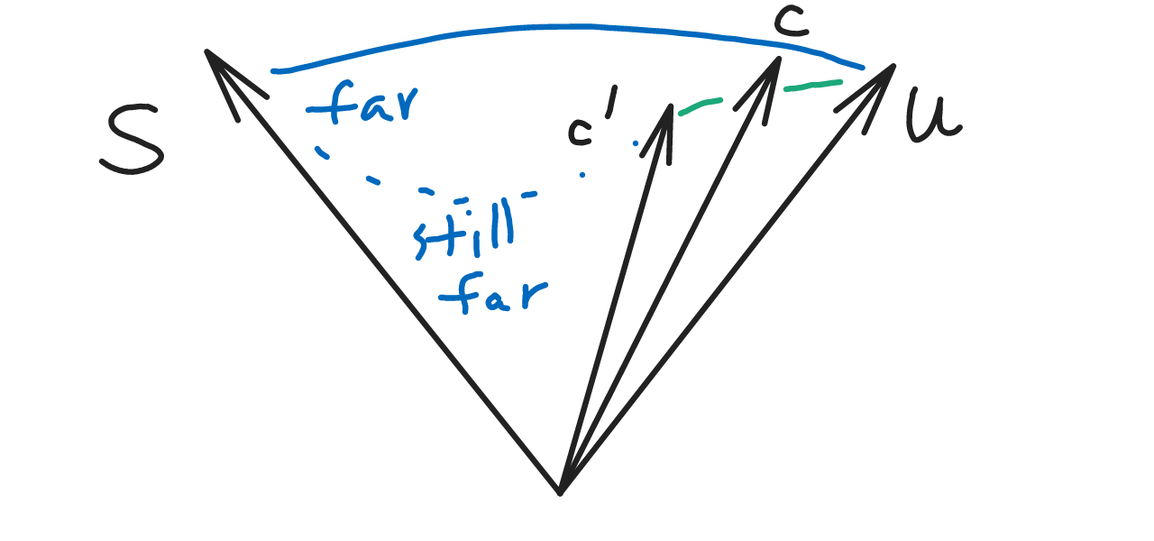
   • Summary of parameters in Theorem 5.1.
     • Running time \(n^{O(k)}\): Just to evaluate \(W\) on a degree \(k\) p.d. takes \(n^{O(k)}\) time.
     • Success probability \(2^{-k/\poly(\ep)}\): \(W\) succeeded if each \(\an{c,\xi^{(i)}}\) is large, so we get \(-k\) in the exponent. (!! This seems like a very crude bound—I expect we can do much better, maybe even subexponential?) \(M\) depends polynomially on \(\rc{\ep}\); \(\rc{\poly(\ep)}\) is in the exponent because the algorithm relies on sampling to get close enough.
3. Finish.
   • In step 1, from 6.1, we get \(\wt \E \an{c,u}^k \ge e^{-\ep' k}\), \(\ep' = O\pa{\fc\tau d+ \fc{\ln \si}d + \fc{\ln m}k}\).
   • From 5.1, we get \(c'\) close to a column \(c\) of \(A\): \(\an{c,c'}\ge 1-O(\ep')\) with probability \(2^{-\fc{k}{\poly(\ep')}}\). Repeat \(2^{\fc{k}{\poly(\ep')}}\) times to get this with good probability. (\(\ep = \Te(\ep')\).)
   • (Far from other vectors already in \(S\)) We have \(P(c') \ge c^Tc' - \tau\ve{c'}_2^2 \ge e^{-\ep d}-\tau\). Calculation using the triangle inequality on (after doing \(\bullet^{\ot 2}\) because the inequality we have is \(\an{s,U}^2\le 1-\ga\)) gives \(\an{c',s}\le 1-\fc{\ga}{10}\). (We chose \(\ga = C\ep\).)
   • (Every \(s\in S\) is close to some column.) Use 6.1 on \(s\) (which is an actual vector! not a p.d.), \(\ve{A^T s}_d^d \ge e^{-\ep d}-2\tau\) to get \(\an{s,c}^2 \ge 1-O(\ep)\).
   • (Can’t have 2 \(s\in S\) close to same \(c\)) More triangle inequalities.
   • The algorithm then terminates after \(|S|=m\). The total time is \(n^{O(k)/\poly(\ep)} = n^{\fc{\ln m}{\poly(\ep)}}\). There’s an extra \(d\) in the exponent because accessing \(P\) takes \(n^d\) time. (CHECK!!)

Dictionary learning

Theorem

The algorithm below, given

• \(\ep>0\)
• overcompleteness \(\si\ge 1\)
• \(d\ge D:=O\pf{\ln \si}{\ep}\),
• \(\tau \le (D\si)^{-D}\). (In 4.2 it says \(D^D\), but I think it should be this.)
• \(\wt O \pf{n^{2d}}{\tau^2}\) samples from \(y=Ax\) for \((d,\tau)\)-nice \(x\),

outputs in time \(n^{\fc{d+\ln m}{\ep^{O(1)}}}\) a set of vectors \(\ep\)-close to \(A\).

Algorithm

Take \(\wt O \fc{n^{2d}}{\tau^2}\) samples \(x^{(i)}\) and apply noisy tensor decomposition to the polynomial \[ \EE_i x^{(i)} \an{Ax,u}^d \] where \(d\ge D:=O(\ep^{-1}\ln \si)\).

Note that \(\an{Ax,u}^d\) is the polynomial (\(n\)-ic form) corresponding to the tensor \((Ax)^{\ot d}\), just as \(u^T vv^Tu = \an{u,v}^2\) is the quadratic form corresponding to the matrix \(vv^T\).

Proof.

1. (Calculate expectation) Lemma 4.5. If the distribution of \(x\) is \((d,\tau)\)-nice and \(A\) is \(\si\)-overcomplete, then \[\EE_x \an{Ax,u}^d \in \ve{A^Tu}_d^d + [0,\tau \si^dd^d \ve{u}_2^d]\] (where inequalities are in the SoS sense).

   Proof. Expand the sum as \(\sum_\al x_\al (A^Tu)_\al\). For \(\al=[i,\ldots, i]\) we get the term \((A^Tu)_i^d\). For the other terms, \[\begin{align} 0 &\le \sum_{\al \in [n]^d,\al \ne [i,\ldots, i] }(\E x_\al) (A^Tu)_\al \\ & \le \tau \sum_{\al \in [n]^d,\al \ne [i,\ldots, i] } (A^Tu)_\al \\ & \le \tau d^d\sum_{\be \in [n]^{d/2},\be \ne [i,\ldots, i] } (A^Tu)_\be\\ & \le \tau d^d\ve{A^Tu}_2^d \le \tau \si^d \ve{u}_2^d. \end{align}\] (The \(d^d\) bound is crude; this is not the bottleneck.) Note the lower inequality depends on there only being even nonzero terms.
2. (Calculate concentration, Proof of 4.2) We use a Chebyshev bound¹. We have \(|(A^Tx)_\al|\le 1\). I think we need assumption on \(\ve{A^Tx}_{\iy}\). Thus taking \(\wt \Om\pf{n^{2d}}{\tau^2}\) samples we get that the coefficients are whp \(\fc{\tau}{n^d}\)-close. This means the value at \(u\) is \(n^d \si^d\fc{\tau}{n^d}\)-close, and we get whp \[P\in \ve{A^Tu}_d^d + 2\tau \si^d d^d \ve{u}_2^d[-1,1].\]

3. Use noisy tensor decomposition. Check parameters. There we needed \(d \ge D=O(\rc{\ep}\ln \si)\). We need \(\tau\le \fc{\ep}{\si^DD^D}\). (Errata? The value of \(\tau\) is different than in the theorem.)

Polytime algorithm

This means polytime for fixed \(\ep\). Note to get \(\rc{\ln n}\) closeness (ex. for initialization of an iterative DL algorithm), we need quasipolytime, \(n^{O(\ln n)}\).

The bottleneck is the \(\ln m\) in Lemma 6.1, where we used averaging to conclude that if \(U\) has large correlation with \(A\), then \(U\) has large correlation with a column of \(A\).

To summarize the previous argument, we show our distribution of \(W\) satisfies inequalities given in 5.2, and then use reweighting to obtain that \(u\) is correlated with some column in 5.1. Now we use the weak lemma 6.1 which recovers that column, with \(\ln m\) loss.

If we weaken the conclusion of 6.1, then we can hope that 6.1’, i.e., 7.3, doesn’t have a \(\ln m\) in the place we care about. Then we need 5.1’, i.e., 7.1, to work with these weaker conditions. Sparsity allows us to weaken the conditions on correlation, provided we have better bounds information about the distribution \(W\) that we choose.

(Not quite: 5.2 was a lemma for 5.1. 7.1 is a lemma for 7.2, we use 7.1+5.1 to get 7.1.)

Specifically, the condition on the p.d. \(U\) (degree \(2(1+2k)\)) is (7.2) \[ \wt \E\an{c,U}^{2(1+2k)} \ge e^{-\ep k} \wt \E \an{c,U}^2, \qquad \wt E\an{c,u}^2\ge \tau^k. \] This is easier to satisfy: the \(\rc m\) that causes problems is moved to the second inequality (as long as we have sparsity \(\tau^k\le \rc m\) we are OK). The second inequality is true if sparsity is \(\tau\) (CHECK!!). \(k\) no longer needs a factor \(\rc{\ln m}\) in the denominator to satisfy this.

Note 5.2, 5.1 don’t mention the sparsity at all, while 7.2, 7.1 mention \(\tau\) which will be related to the sparsity.

Some changes: instead of reducing from degree \(k\) to \(2\) we reduce from degree \(\approx 4k\) to \(2k\). (??)

So how does the algorithm work now, given that our assumption is (7.2) rather than a bound on \(\wt \E \an{c,u}\)? 7.1 has the following inequality on \(\ol W= \E_WW\), (7.1): \[\an{c,U}^{2(1+k)}\preceq \ol W \preceq (\an{c,U}^2 + \tau\ve{U}_2^2)^{1+k}.\] Using this, get an upper bound on \(\wt \E \ol W\) and lower bound on \(\wt \E \an{c,U}^{k}\) to get a lower bound on \(\wt\E \ol W\an{c,U}^{2k}\): \[\wt \E \ol W\an{c,U}^{2k} \wt \E \ol W \ge [\wt \E(\ol W \an{c,U}^k)]^2.\]

The bound on \(\ol W\) comes from sparsity. Take \(W=\prodo i{k/2-1} \an{y_i=Ax_i,U}^2\). \(\ol W\) does not actually satisfy (7.1); it does after reweighting by \(\prodo i{k/2-1} x_{i,1}^2\). (This is a distribution over polynomials. Take the probability that \(\prod \an{Ax_i,U}^2\) is chosen and multiply it by \(\prod x_{i,1}^2\) and normalize the probabilities. (Not multiply the polynomial.)) Consider \(c\an{Ax,u}^2\) reweighted by \(x_i^2\); expand and use sparsity to get a nice bound on expectations.

This is much better than the previous analysis on \(W\)! It actually seems to take into account some kind of concentration…

Final theorem is 7.6.

Todo

• Summarize changes to get down to polytime. What’s the key idea?

(Q: can you adapt something like this for NMF?)