PMI for images

Posted: 2016-08-01 , Modified: 2016-09-15

Results

Results

Summary

Distribution of PMI of pairs of features has a longer tail than a Gaussian.
Restricting to one digit (conditional PMI) does not increase the PMI much, except for the digit 1, which has very large CPMI compared to all other digits.
Pairs of features with large PMI are more likely (weakly) to have large activation with the same digit.
Feature vectors are close to sparse. (See “PMI suitability” below.)
Call a feature discriminative if its maximum average activation with a digit is \(\ge 0.1\) and is \(\ge 1.5\) times the average activation with the second most activated digit. There are 2080/7200 discriminative features, but only 155 of them do not correlate most strongly with “1”, and some digits are not represented at all.
The maximum PMI (between a pair) is 2.69. However, the largest PMIs actually come from pairs with small maximum activation. If we remove all features that do not have an activation of \(\ge 0.5, 1.0\) in some image, then the maximum PMI is 2.16, 1.79.
The learned SVM have both positive and negative weights. (The distribution of weights is roughly symmetric.)
Running SVM on the 500-dimensional SVD of the feature vectors results in performance that is as good as SVM on the feature vectors.
(Local SVD) Taking the 12-dimensional SVD of each of the 36 patches (either together or separately) (which reduces dimension to 432) results in similar performance.
Weighted SVD does not increase accuracy, though it seemed to make training faster in the local SVD experiment.
Some features from the same/adjacent patches have large PMI, but many (most) pairs with large PMI are not close by geometrically.
Most features do not have large activation with only one digit.

Distribution of PMI pairs

CODE: First calculate psiTr. (It has been saved as data/psiTr_1.mat.) Then run calculate_cpmi_unnormalized_script.

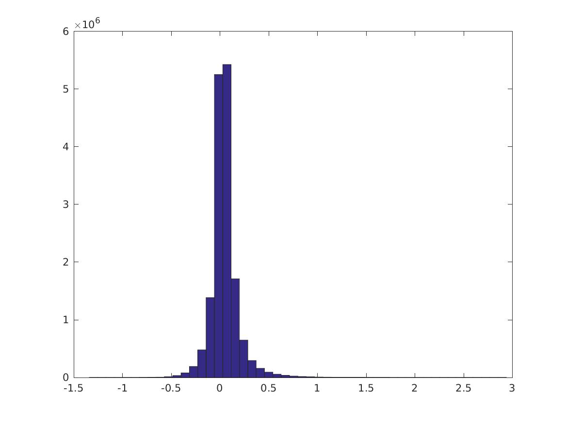
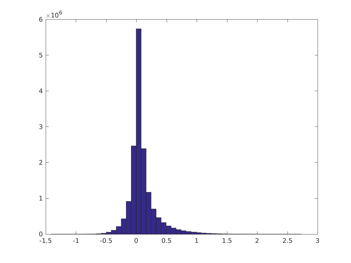
Over all pairs of nonzero features \(\{i,j\}\), this is the distribution of \(PMI(v_i,v_j)\). Note the long tails. Here we don’t normalize the features first. (You can also try with various normalizations, by passing in a normalization function to calculate_cpmi_unnormalized.) There are 5652/7200 nonzero features.

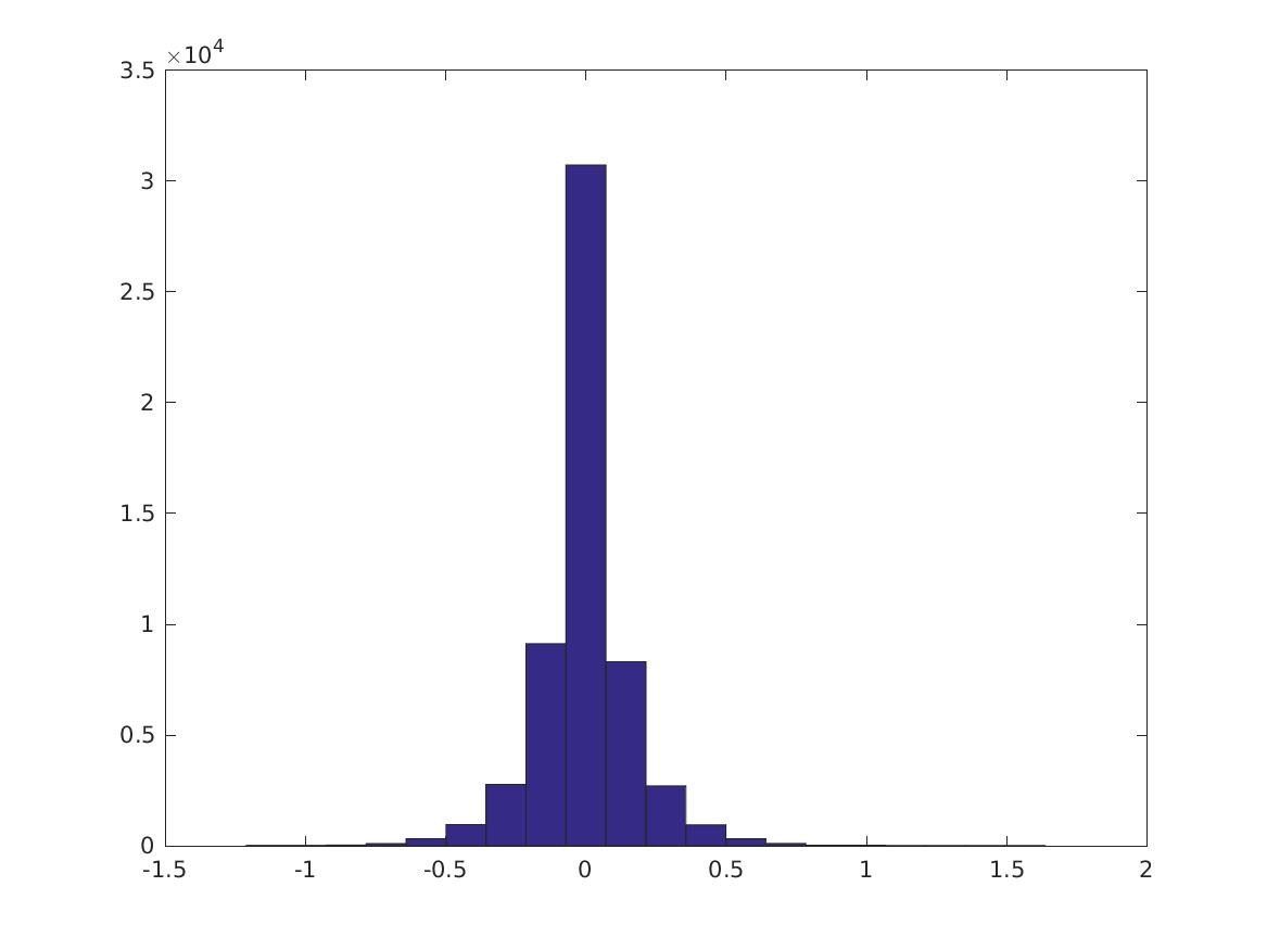
Conditioned on the digit being a specific value, how does the PMI distribution look? Still about the same… except that 1 has much larger activation. These are digits 0-9 in order.

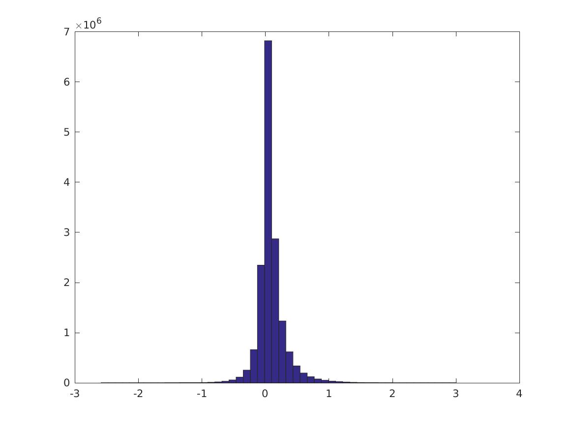
Here are the 0, 10,…, 100 percentiles of these distributions. The first 10 rows are the CPMI distributions for digits 0-9; the last row is the PMI distribution. It’s not always true that the CPMI’s for a digit are larger.

  Columns 1 through 7

   -1.3409   -0.0831   -0.0288   -0.0008    0.0178    0.0340    0.0520
   -3.4897   -0.4067   -0.1484   -0.0196    0.0449    0.1054    0.1912
   -1.2622   -0.1009   -0.0318    0.0013    0.0221    0.0404    0.0618
   -1.3727   -0.0931   -0.0249    0.0067    0.0265    0.0458    0.0705
   -2.5869   -0.0910   -0.0227    0.0091    0.0304    0.0524    0.0804
   -1.4005   -0.0930   -0.0239    0.0113    0.0353    0.0582    0.0857
   -2.6503   -0.0855   -0.0157    0.0134    0.0334    0.0555    0.0847
   -3.1251   -0.1389   -0.0498   -0.0046    0.0237    0.0488    0.0796
   -1.4074   -0.0984   -0.0277    0.0047    0.0240    0.0436    0.0701
   -2.7278   -0.0846   -0.0149    0.0156    0.0372    0.0624    0.0966
   -1.1984   -0.0727   -0.0094    0.0253    0.0534    0.0847    0.1241

  Columns 8 through 11

    0.0754    0.1111    0.1828    2.9385
    0.3236    0.5373    0.9549    5.9331
    0.0911    0.1378    0.2326    1.9094
    0.1069    0.1677    0.2931    1.8452
    0.1201    0.1838    0.3111    3.0054
    0.1236    0.1841    0.3266    3.0518
    0.1286    0.2034    0.3556    3.7582
    0.1237    0.1959    0.3409    3.2767
    0.1110    0.1844    0.3448    2.7204
    0.1484    0.2350    0.4080    3.4744
    0.1778    0.2587    0.4034    2.6897

Thresholding by psiTr

CODE: Run top_pmis_script which runs pmi_threshold_f and check_top_pmis_f.

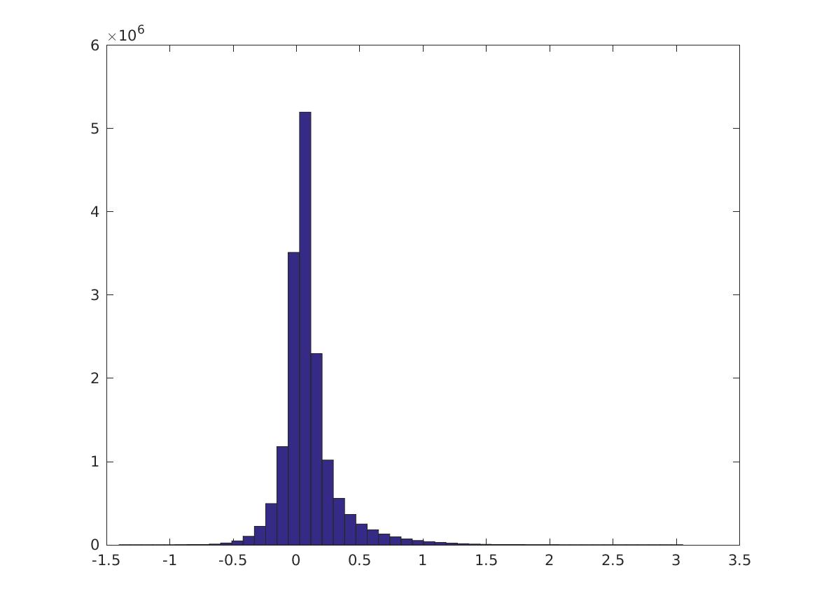
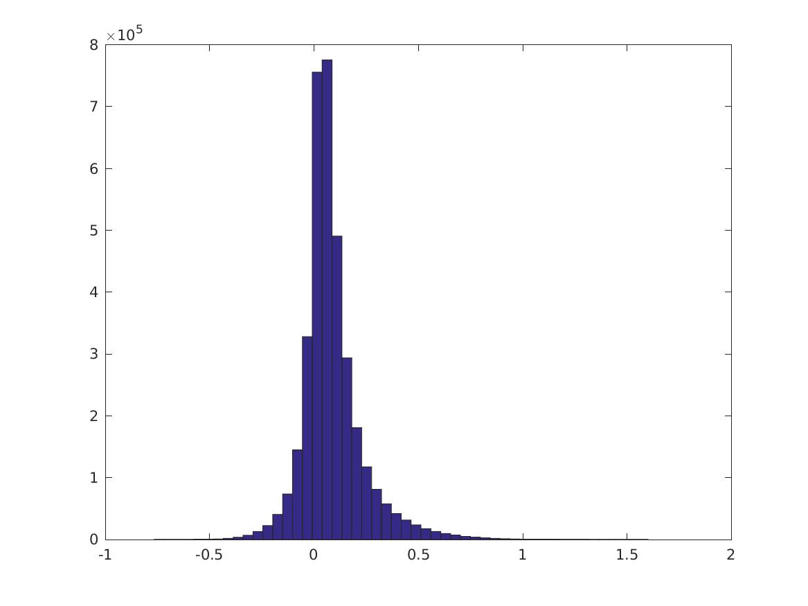
Remove all features that do not have activation \(>1\) in some image. Now do the same thing. (NOTE: the maximum PMI is less because the max PMI’s are between features that have small maximum activation. Try this again thresholding by PMI?)

This is the distribution of \(PMI(v_i,v_j)\):

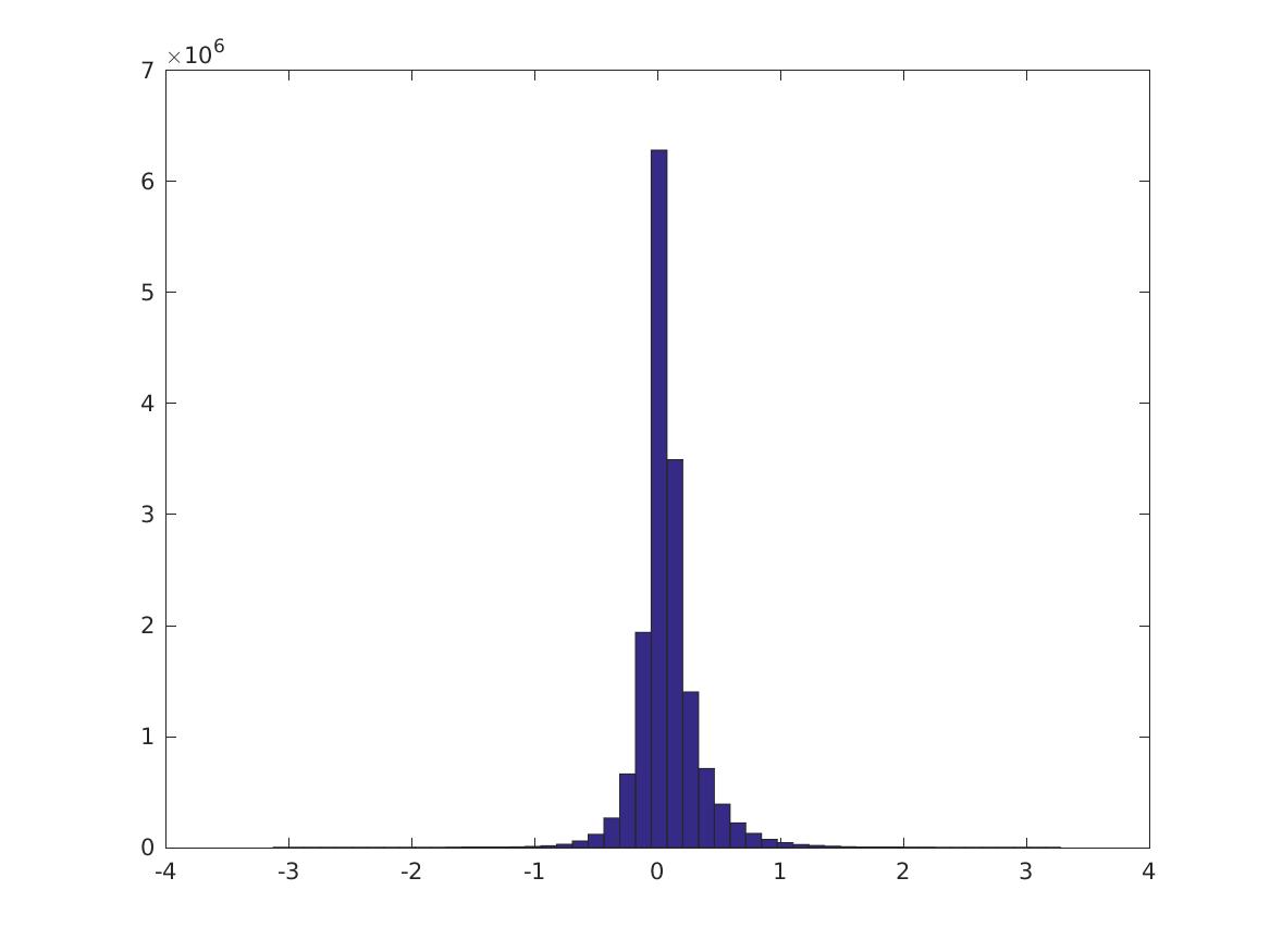
These are digits 0-9.

Percentiles of the distributions (\(i\)th row is 0, 10, 20, … 100% for the CPMI’s of digit \(i\), last row is PMI over all digits). (Note the last column is different)

  Columns 1 through 7

   -0.9746   -0.0588   -0.0140    0.0112    0.0306    0.0488    0.0681
   -3.1365   -0.3102   -0.0940    0.0050    0.0609    0.1144    0.1812
   -0.9300   -0.0626   -0.0130    0.0134    0.0333    0.0526    0.0740
   -0.7660   -0.0462   -0.0022    0.0210    0.0403    0.0602    0.0835
   -2.0740   -0.0565   -0.0071    0.0188    0.0397    0.0611    0.0855
   -0.8674   -0.0628   -0.0077    0.0229    0.0471    0.0705    0.0966
   -2.3770   -0.0457   -0.0007    0.0228    0.0428    0.0639    0.0886
   -2.4824   -0.0928   -0.0235    0.0121    0.0379    0.0633    0.0925
   -0.9435   -0.0521   -0.0066    0.0161    0.0347    0.0545    0.0785
   -2.1549   -0.0505   -0.0020    0.0231    0.0446    0.0679    0.0961
   -0.8693   -0.0515    0.0008    0.0344    0.0640    0.0949    0.1309

  Columns 8 through 11

    0.0910    0.1215    0.1730    1.5181
    0.2772    0.4314    0.7470    5.3609
    0.1007    0.1393    0.2117    1.5297
    0.1141    0.1604    0.2521    1.6011
    0.1169    0.1635    0.2537    2.2486
    0.1293    0.1773    0.2773    2.0363
    0.1215    0.1727    0.2771    2.5443
    0.1305    0.1882    0.3019    2.9006
    0.1111    0.1639    0.2788    2.1102
    0.1344    0.1957    0.3210    2.7701
    0.1761    0.2406    0.3557    1.7908

check_top_pmis produces a graph showing which features are close to each other. It’s not very enlightening.

PMI suitability

CODE: Run pmi_suitability.m.

Is PMI the right measure? Are the feature vectors close to sparse? if the average image there is \(>20\%\) activation, then no.

For the first 10 images, this is what the percentiles look like:

percentiles:

pcs =

   100    99    95    90    80    70

Image 1 (label 5)
    2.3230
    1.2966
    0.8840
    0.6766
    0.4381
    0.3140

Image 2 (label 0)
    2.1275
    1.3604
    0.9482
    0.7418
    0.5036
    0.3769

Image 3 (label 4)
    1.7975
    0.9874
    0.6185
    0.4704
    0.3145
    0.2247

Image 4 (label 1)
    2.2506
    1.2399
    0.7160
    0.4949
    0.3029
    0.1992

Image 5 (label 9)
    2.0837
    1.3970
    0.8726
    0.6461
    0.3937
    0.2707

Image 6 (label 2)
    2.4831
    1.4978
    1.0466
    0.7880
    0.5002
    0.3544

Image 7 (label 1)
    2.5064
    1.3688
    0.7591
    0.5203
    0.3089
    0.1935

Image 8 (label 3)
    3.3030
    1.6943
    1.1588
    0.8658
    0.5756
    0.4070

Image 9 (label 1)
    2.2263
    0.9396
    0.4905
    0.3279
    0.1944
    0.1178

Image 10 (label 4)
    2.2420
    1.3486
    0.8494
    0.6169
    0.3751
    0.2586

This looks pretty good—the top 1% of features are much larger than the rest.

Look for discriminative features, those that occur with one label and rarely for others. (I arbitrarily define this as: the maximum average activation is \(>1.5\) times the second largest, and the maximum is at least 0.1. I exclude the digit 1 (indexed as 2).)

sig_act_inds = intersect(find(m1>=1.5*m2), find(m1>0.1));
sig_act_inds2 = intersect(sig_act_inds, find(am1 ~=2));

2080/7200 features fit the first criteria, 115/7200 of them are not 1. The distribution across labels is

Some labels are not represented!

SVD-SVM

Do SVM coefficients have negative weights?

They have both positive and negative weights.

>> size(find(coeffs>0))

ans =

           1       26333

>> size(find(coeffs<0))

ans =

           1       30187

CODE: Run svd_testing2.m, or sbatch slurm_svd.cmd. The results are saved in accs_1.mat.

Results:

Dimension	Last	Best
Original	99.34	99.44
500	99.26	99.44
100	97.5	98.82
50	96.84	96.84

Weighted SVD-SVM

Do weighted SVD (as in the NLP paper) and then train a SVM. Note this does worse than just SVD! Why?

Dimension	Last	Best
50	95.44	96.8

Local SVD

CODE: Run local_svd_svm.m and local_wsvm_script1.m.

Four settings:

Run SVD with dimension 12 for each patch separately.
Run SVD with dimension 12 for patches collectedly.
Run WSVD with dimension 12 for each patch separately.
Run WSVD with dimension 12 for patches collectedly.

(Dimension \(36\times 12 = 432\) total.)

Type	Last	Best
SVD, separately	99.18	99.24
SVD, collected	99.34	99.34
WSVD, separately	99.1	98.7
WSVD, collected	99.2	99.2

The training is stored in ../data/local_SVD.mat (got overridden, unfortunately) and ../data/local_wsvd_collected.mat.

One instance of training collected SVD.

accVal =

  Columns 1 through 7

   85.6800   85.6800   85.6800   85.6800   85.7200   85.9200   85.9400

  Columns 8 through 14

   86.3400   87.1600   87.9600   89.3800   91.2400   92.6200   94.1400

  Columns 15 through 21

   95.3400   96.1400   96.8600   97.3200   97.8400   98.1200   98.4800

  Columns 22 through 28

   98.5800   98.8400   98.8600   98.9200   98.9600   99.0600   99.1600

  Columns 29 through 31

   99.1800   99.3000   99.2000

WSVD, separate

  Columns 1 through 7

   92.1800   93.9200   95.0400   95.9400   96.6800   97.3400   97.8600

  Columns 8 through 14

   98.2200   98.4000   98.5800   98.7000   98.7600   98.9000   99.0000

  Columns 15 through 21

   99.0600   99.0400   99.0000   98.8600   99.1000   98.8800   98.3400

  Columns 22 through 28

   99.0000   98.9000   98.1600   98.9200   98.8200   99.0200   98.9800

  Columns 29 through 31

   98.9200   98.9600   98.7000

PMI and geometry

CODE: Run geo_pmi.m.

Hypothesis: The largest PMI values are for features that are for the same patch or adjacent patches.

The features are in a \(6\times 6\) grid; each of the 36 patches have a total of 200 features. We calculate the following PMI’s:

Collect all the patches together, so we only have 200 features.
Calculate PMI’s between pairs in the same patch. (without collecting, so 7200 features)
Collect patches together, and calculate PMIs between each feature and the same feature translated right 1 patch.
Calculate PMI’s only between pairs in horizontally adjacent patches.
Collect patches together, and calculate PMIs between each feature and the same feature translated down 1 patch.
Calculate PMI’s only between pairs in vertically adjacent patches.
All PMI’s.

The collection process reduces the PMI’s. It seems that many of the largest PMI’s do occur in the same or adjacent patch.

collect, same patch; no collect, same patch; horiz collect; horiz no collect; vert collect; vert no collect; all

ans =

  Columns 1 through 7

   -0.9605   -0.3457   -0.2067   -0.1000   -0.0103    0.0783    0.1698
   -1.0872   -0.0690   -0.0062    0.0281    0.0563    0.0880    0.1277
   -1.5676   -0.3858   -0.2386   -0.1310   -0.0454    0.0409    0.1303
   -0.9235   -0.0241    0.0307    0.0621    0.0919    0.1266    0.1695
   -1.3763   -0.3810   -0.2237   -0.1053   -0.0072    0.0839    0.1708
   -0.9163   -0.0108    0.0284    0.0530    0.0796    0.1093    0.1458
   -1.1984   -0.0727   -0.0094    0.0253    0.0534    0.0847    0.1241

  Columns 8 through 11

    0.2735    0.3922    0.5678    1.3093
    0.1821    0.2624    0.4080    2.4518
    0.2220    0.3257    0.4557    1.1007
    0.2240    0.3054    0.4534    2.6332
    0.2607    0.3593    0.4863    0.9118
    0.1942    0.2660    0.3970    2.6332
    0.1778    0.2587    0.4034    2.6897

Are the largest PMI’s close together?

No.

Pairs with large PMI aren’t necessarily adjacent. These are the top few PMI’s, with \((x_1,y_1), (x_2,y_2),\ve{(x_1,y_1)-(x_2,y_2)}\) (locations within the grid). (The following data is without thresholding and excluding 1’s; with thresholding it also looks similar.)

    3.0000    4.0000    1.0000    1.0000    3.6056
    1.0000    6.0000    1.0000    1.0000    5.0000
    3.0000    5.0000    1.0000    1.0000    4.4721
    2.0000    2.0000    1.0000    6.0000    4.1231
    2.0000    2.0000    1.0000    1.0000    1.4142
    1.0000    4.0000    1.0000    1.0000    3.0000
    1.0000    1.0000    1.0000    1.0000         0
    1.0000    4.0000    1.0000    1.0000    3.0000
    3.0000    3.0000    1.0000    1.0000    2.8284
    4.0000    5.0000    1.0000    1.0000    5.0000

Largest PMIs

I sorted pairs of features by PMI value and took the largest 10000 pairs. The majority of the pairs (~77%) have strongest activation with the digit 1. (The digit 1 has conditional PMI values that are much larger than all the other digits - don’t know what to do about this.) 85% of the pairs have highest activations with the same digit.

If the pair has strong activation with 1, then it’s often much larger than the other activations.

Otherwise this is not necessarily true. A typical non-1 feature has average activations with the 10 digits that looks something like this: (NOTE: This was normalized—run again unnormalized to match the rest of the data.)

  Columns 1 through 7

    0.0708    0.2673    0.0940    0.1537    0.2122    0.1116    0.2627

  Columns 8 through 10

    0.2947    0.1448    0.3361