Basic information
This page is about the following paper:
Ge, R., Lee, H., & Risteski, A. (2018). Beyond Log-concavity: Provable Guarantees for Sampling Multi-modal Distributions using Simulated Tempering Langevin Monte Carlo. NIPS AABI workshop 2017 and NIPS 2018. arXiv preprint arXiv:1812.00793.
- arXiv, pdf.
- A previous version of the paper, with a more complicated proof and weaker result, appeared in NIPS AABI workshop 2017, and is on arxiv here.
- Slides
- Poster
- 3 minute video
- Blog post on Off-Convex: part 1, part 2.
Abstract
A key task in Bayesian statistics is sampling from distributions that are only specified up to a partition function (i.e., constant of proportionality). However, without any assumptions, sampling (even approximately) can be #P-hard, and few works have provided “beyond worst-case” guarantees for such settings. A key task in Bayesian statistics is sampling from distributions that are only specified up to a partition function (i.e., constant of proportionality). However, without any assumptions, sampling (even approximately) can be #P-hard, and few works have provided “beyond worst-case” guarantees for such settings.
For log-concave distributions, classical results going back to Bakry and Emery (1985) show that natural continuous-time Markov chains called Langevin diffusions mix in polynomial time. The most salient feature of log-concavity violated in practice is uni-modality: commonly, the distributions we wish to sample from are multi-modal. In the presence of multiple deep and well-separated modes, Langevin diffusion suffers from torpid mixing.
We address this problem by combining Langevin diffusion with simulated tempering. The result is a Markov chain that mixes more rapidly by transitioning between different temperatures of the distribution. We analyze this Markov chain for the canonical multi-modal distribution: a mixture of gaussians (of equal variance). The algorithm based on our Markov chain provably samples from distributions that are close to mixtures of gaussians, given access to the gradient of the log-pdf.
Blog post
In this post I describe recent work with Rong Ge and Andrej Risteski on an algorithm that provably samples from certain multimodal distributions.
Sampling is a fundamental task in Bayesian statistics, and dealing with multimodal distributions is a core challenge. One general approach to sample from a probability distribution is to define a Markov chain with the desired distribution as its stationary distribution. This approach is called Markov chain Monte Carlo. However, in many practical problems, the Markov chain does not mix rapidly, and we obtain samples from only one part of the distribution.
Practitioners have dealt with this problem through heuristics involving temperature. However, there has been little theoretical analysis of such methods. In our paper, we give provable guarantees for a temperature-based method called simulated tempering when it is set up correctly with the base Markov chain, called Langevin diffusion.
Here is a cartoon of our results:
Cartoon
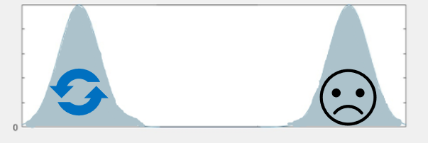
A Markov chain with local moves such as Langevin diffusion gets stuck in a local mode.
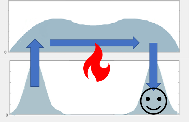
Creating a meta-Markov chain which changes the temperature can exponentially speed up mixing.
Problem
The concrete problem we address is the following.
Sample from a probability distribution \(p(x) \propto e^{-f(x)}\), \(x\in \R^d\) given access to \(f(x)\) and \(\nabla f(x)\).
We can’t hope to solve this problem in full generality1, but we can hope to find methods that work for a wider class of distributions, including some multimodal distributions.
Introduction
First I give some background for the problem.
- I’ll explain the analogy between sampling and optimization, in particular how going beyond convexity in optimization is like going beyond log-concavity in sampling.
- I’ll describe some connections between sampling and optimization, hopefully motivating people who work in optimization to care about sampling.
Optimization vs. sampling
The great divide of optimization
The goal in optimization is to find the minimum of a function \(f\).
When \(f\) is convex, this is well-understood:
- There is a unique local minimum, which is a global minimum.
- This allows local search algorithms such as gradient descent (as well as a whole extended family of zero, first, and second order algorithms) to work.
- Well-established mathematics characterizes how fast we can optimize convex functions based on various properties.
On the other hand, when \(f\) is non-convex,
- There can be many bad local minima.
- Gradient descent can get trapped in those local minima.
- The problem is NP-hard in the worst-case. This is a barrier for theoreticians as it means we won’t have clean, beautiful, assumption-free results, and we’ll have to get our hands dirty.
- Still, gradient descent-like algorithms often still well in practice.
This is the “great divide” in optimization. On one side we have the well-understood area of convex optimization, and on the other we lump everything under the label “non-convex”. We care about non-convex optimization because many practical optimization problems (such as those arising in machine learning, and deep learning in particular) are very non-convex. In light of the worst-case results we’ll have to get our hands dirty and see what is the structure of real-world problems that allow us to do nonconvex optimization, to close the gap between theory and practice.
The great divide of sampling
Analogously we have a “great divide” in sampling.
Recall that we want to sample from \(p(x)\propto e^{-f(x)}\) where \(x\in \R^d\). When \(f\) is convex, i.e. \(p\) is log-concave, this is well-understood.
- \(f\) has a unique local minimum, which means the distribution \(p\) is unimodal.
- There is a natural algorithm (a Markov chain) called Langevin diffusion - which is basically gradient descent plus gaussian noise - that works, and a lot of beautiful math that goes into the analysis.
On the other hand, when \(f\) is non-convex,
- \(p\) can be multimodal
- Langevin diffusion can take exponentially long to mix, because it gets trapped in one of the modes.
- The problem is #P-hard in the worst case.
- Sampling algorithms can still do well in practice, sometimes with the aid of heuristics such as temperature-based methods.
We care about this difficult case because modern sampling problems (such as those arising in Bayesian machine learning) are often non-log-concave. Like in nonconvex optimization, we must go beyond worst case analysis, and find what kind of structure in non-log-concave distributions allows us to sample efficiently.
Note that log-concavity makes sense for sampling problems on \(\R^d\), but there are other conditions that similarly give guarantees for mixing, such as correlation decay for problems in \(\{0,1\}^d\). As is the case for log-concavity, we have provable guarantees for problems satisfying correlation decay, and beyond it, the field is murkier.
Why optimizers care about sampling
The primary connection between optimization and sampling is the following: if we sample from \(e^{-f}\), we’re more likely to get points where \(f\) is small. We can take this to the extreme: In the limit as \(\beta \to \infty\), the distribution \(e^{-\beta f}\) is peaked at exactly the global minima. \(\beta\) is called the inverse temperature (\(\beta=\frac 1T\)) in statistical physics.
So in a sense, optimization is “just” a sampling problem. In reality, however, we can’t usually take \(\beta\to \infty\), so there is tradeoff between ability to sample and quality of the solution.
Here is a list of past work connecting optimization and sampling, or more generally, using randomness:
- To escape local minima, we can add noise to gradient descent (which is exactly Langevin diffusion), at the cost of not exactly getting a minimum. This has been analyzed in, for example, A hitting time analysis of stochastic gradient langevin dynamics. 2
- Several works have heuristically explained the success of stochastic gradient descent using Langevin dynamics: if we pretend the noise from the stochasticity is gaussian, then we get exactly Langevin dynamics and the ability to escape local minima. The noise can also be thought of as imposing a prior, helping generalization.
- Langevin dynamics has also inspired temperature-based methods such as entropy-SGD for optimizing neural networks.
- Other works on non-convex optimization also use the idea of randomness, for example, adding perturbations to help escape saddle points. See post.
- Another connection to note is a work by Jake Abernathy and Elad Hazan connecting the interior point methods (following the central path) to simulated annealing for convex optimization. See post.
Main result
We analyze a natural algorithm for sampling beyond log-concavity, combining Langevin diffusion with simulated tempering. We show efficient sampling given a structural assumption on the distribution, that it is close to a mixture of gaussians with polynomially many components.
Our main theorem is the following.
Theorem: Let \(p(x)\propto e^{-f(x)}\) be a mixture of gaussians, i.e., \[f(x)=-\ln\pa{\sumo in w_i e^{-\fc{\ve{x-\mu_j}^2}{2\si^2}}}\]. Suppose we can query \(f(x)\), \(\nb f(x)\), and \(\si, \ve{\mu_j}\le D\). There is an algorithm (based on Langevin diffusion and simulated tempering), which runs in time \(\poly(1/w_{\min},1/\si^2,1/\ep,d,D)\) that samples from a distribution \(\wt p\) with \(\ve{p-\wt p}_1\le \ep\).
Moreover, this theorem is robust in the following sense: if \(f\) is only \(\De\)-close in \(L^{\iy}\) distance to a mixture of gaussians, then we incur an additional factor of \(\poly(e^{\De})\) in complexity.
Algorithm
The two algorithmic tools are
- Langevin diffusion, which is a generic chain for sampling given gradient access to log-pdf of distribution, and
- Simulated tempering, a heuristic for speeding up Markov Chains on multimodal distributions.
Langevin diffusion
Langevin is a continuous time random-walk for sampling from \(p\propto e^{-f}\), given access to the gradient of the log-pdf, \(f\). It is gradient flow plus Brownian motion, and described by a stochastic differential equation \[dx_t = -\be_t \nb f(x_t)dt + \sqrt 2 d W_t.\] It’s not necessary to understand the stochastic calculus: you can think of this as the limit of a discrete process, just as gradient flow is the continuous limit of gradient descent. The \(\eta\)-discretized version is where we take a gradient step, with step size \(\eta\), and add gaussian noise scaled by \(\sqrt{2\eta}\):3 \[x_{t+\eta}=x_t-\eta \nb f(x_t) + \sqrt{2\eta}\xi_t.\]
Langevin diffusion has been well-studied, both in the math and CS communities. It is a classical result that the stationary distribution is proportional to \(e^{-f(x)}\). Bakry and Emery showed in the 80’s that if \(p\) is \(\alpha\)-log-concave, then the mixing time is on the order of \(\frac 1{\alpha}\) (see Terence Tao’s blog post).
With the recent algorithmic interest in Langevin diffusion, we want similar guarantees for discretized chain - that it converges to a measure close to \(p\). This was done by Dalalyan and Durmus and Moulines, and by Bubeck, Eldan, and Lehec, who also considered restriction to a convex set. For general distributions \(p\) with some regularity conditions, Raginsky, Rakhlin, and Telgarsky showed that there is convergence to \(p\) in time comparable to continuous dynamics.
So why can’t we just run Langevin dynamics?
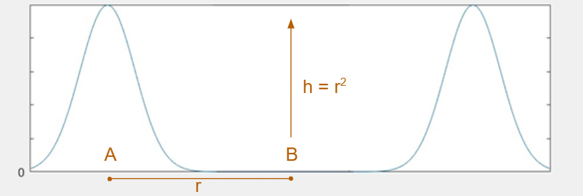
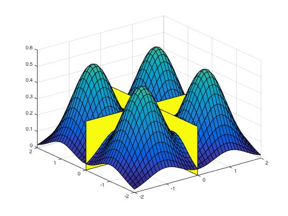
Consider the example of well-separated gaussians. Bovier showed, via the theory of metastable processes, that transitioning from one peak to another takes exponential time. Roughly speaking, to estimate the expected time to travel from one mode to the other, consider paths between those modes. The time will be inversely proportional to the largest possible minimum probability on one of those paths.
If two gaussians with unit variance have means separated by \(2r\), then any path between them will pass through a point with probability less than \(e^{-r^2/2}\), so it will take on the order of \(e^{r^2/2}\) time to move between the gaussians. Think of this as a “energy barrier” Langevin diffusion has to cross. Even if \(r\) is as small as \(\log d\), the time will be superpolynomial in \(d\).
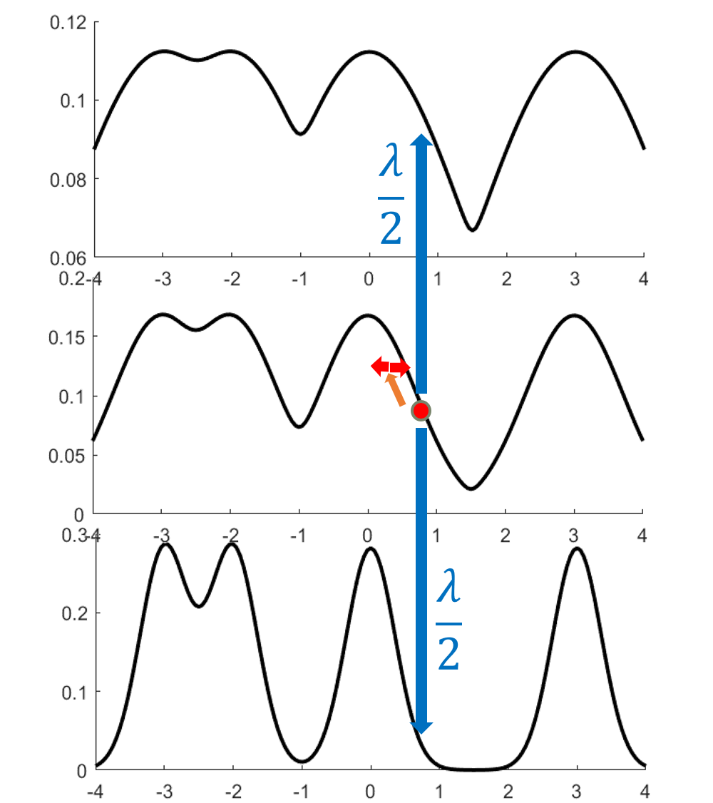
Simulated tempering turns the heat on
A key observation is that Langevin corresponding to a higher temperature distribution (with \(\beta f\) rather than \(f\), where \(\beta<1\)) mixes faster. A high temperature flattens out the distribution.4
However, we can’t simply run Langevin at a higher temperature because the stationary distribution is wrong. The idea behind simulated tempering is to combine Markov chains at different temperatures, sometimes swapping to another temperature to help lower-temperature chains explore.
We can define simulated tempering with respect to any sequence of Markov chains \(M_i\) on the same space. Think of \(M_i\) as the Markov chain corresponding to temperature \(i\), with stationary distribution \(\propto e^{-\beta_i f}\).
Then we define the simulated tempering Markov chain as follows.
- The state space is \(L\) copies of the state space (in our case \(\mathbb R^d\)), one copy for each temperature.
- The evolution is defined as follows.
- If the current point is \((i,x)\), then evolve according to the \(i\)th chain \(M_i\).
- Propose swaps with some rate \(\lambda\).5 When a swap is proposed, attempt to move to a neighboring chain, \(i'=i\pm 1\). With probability \(\min\{p_{i'}(x)/p_i(x), 1\}\), the transition is successful. Otherwise, stay at the same point. This is a Metropolis-Hastings step; its purpose is to preserve the stationary distribution.
It’s not too hard to see that the stationary distribution is the mixture distribution, i.e., \(p(i,x) = \rc L p_i(x)\). Simulated tempering is popular in practice along with other temperature-based methods such as simulated annealing, parallel tempering, (reverse) annealed importance sampling, and particle filters. Zheng and Woodard, Schmidler, and Huber gave decomposition results that can be used to bound mixing time; however in our setting their bound on mixing time is exponential in the number of gaussians.6
Combining Langevin diffusion and simulated tempering
Our algorithm is the following. Assume \(\sigma=1\) for simplicity.
Take a sequence of \(\beta\)’s starting from \(1/D^2\), going up by factors of \(1+1/d\) (where \(d\) is the ambient dimension) up to 1 and run simulated tempering for Langevin on these temperatures, suitably discretized. Finally, take the samples that are at the \(L\)th temperature.
Proof sketch
There are four main steps in the proof.
- Prove a Markov chain decomposition theorem for distributions, that upper-bounds the mixing time. For discrete/continuous-time Markov chains, this is equivalent to showing a spectral gap/Poincaré inequality.
- Show that the conditions of the theorem are satisfied: mixing on component chains, and mixing on a certain projected chain. This shows that the simulated tempering chain mixes, if we move the \(\beta_i\)’s “inside” the mixture of gaussians. This makes the stationary distribution \(\wt p_i\) at each temperature a mixture of gaussians, so is easier to analyze.
- Show that \(\wt p_i\) are close to the acutal distributions \(p_i\), so that we also have rapid mixing for the original chain.
- Some technical details remain that we won’t cover: bounding the error from discretizing the chain, and estimating the partition functions to within a constant factor.
Markov chain decomposition theorem
Previous decomposition theorems
Madras and Randall’s theorem says that if a Markov chain M mixes rapidly when restricted to each set of the partition, and the “projected” Markov chain mixes rapidly, then M mixes rapidly. The formal statement is the following.
Theorem (Madras, Randall 02): For a (discrete-time) Markov chain \(M\) with stationary distribution \(p\) and a partition \(\Om = \bigsqcup_{j=1}^m A_j\) of its state space, \[\text{Gap}(M) \ge \rc 2 \text{Gap}(\ol M) \min_{1\le j\le m} (\text{Gap}(M|_{A_j})).\]
The projected chain \(\overline M\) is defined on \(\{1,\ldots, m\}\), and transition probabilities are given by average probability flows between the corresponding sets. More precisely, the probability of transitioning from \(j\) to \(k\) is as follows: pick a random point in \(A_j\), run the Markov chain for one step, and see what’s the probability of landing in \(A_k\).
This gives a potential plan for the proof. Given a mixture of \(m\) gaussians, suppose we can partition \(\mathbb R^d\) into \(m\) parts - maybe one centered around each gaussian - such that Langevin mixes rapidly inside each set. Choose the highest temperature so that Langvein mixes well on the entire space \(\R^d\) at that temperature.
Then if the projected chain also mixes rapidly, this proves the main theorem. Intuitively, the projected chain mixes rapidly because the highest temperature acts like a bridge. There is a reasonable path from any component to any other component passing through the highest temperature.
There are many issues with this approach. The primary problem is defining the partition. While there is a way to make this work, we found a simpler proof with better bounds, which I’ll now describe.
Decomposition theorem with sets
The insight is to work with distributions rather than sets.
There’s an idea in math that a theorem is true for sets, then it’s a special case of a theorem for functions - because sets just correspond to indicator functions.
For simulated tempering Langevin on a mixture of Gaussians, we don’t naturally have a decomposition of the state space, we do have a natural decomposition of the stationary distribution - namely the components of the mixture! Think of this as a “soft partition”.
So instead of partitioning \(\Omega\), we decompose the Markov chain and stationary distribution. We prove a new Markov chain decomposition theorem that allows us to do this.
Theorem: Let \(M_{\text{st}}\) be a simulated tempering Markov chain (with stationary distribution \(p\)) made up of Markov chains \(M_i,i\in [L]\). Suppose there is a decomposition \[M_i(x,y)=\sum_{j=1}^mw_{ij}M_{ij}(x,y)\] where \(M_{ij}\) has stationary distribution \(p_{ij}\). If each \(M_{ij}\) mixes in time \(C\) and the projected chain mixes in time \(\ol C\), then the simulated tempering chain mixes in time \(O(C(\ol C +1))\).
The projected chain is defined by \[\begin{align} L((i,j),(i,j')) &= \begin{cases} \fc{w_{i,j'}}{\chi^2_{\text{sym}}(p_{i,j}||p_{i,j'})},&i=i'\\ \fc{\min\bc{\frac{w_{i',j}}{w_{i,j}},1}}{\chi^2_{\text{sym}}(p_{i,j}||p_{i',j'}))} ,&i'=i\pm 1\\ 0,&\text{else.} \end{cases} \end{align}\]where \(\chi^2_{\text{sym}}(p||q)=\max\{\chi^2(p||q),\chi^2(q||p)\}\) is the “symmetrized” \(\chi^2\) divergence.
This theorem is where most of the magic lies, but it is also somewhat technical; see the paper for details.
Applying the decomposition theorem
We consider simulated tempering Langevin diffusion for \[ \wt p_i \propto \sumo jm w_j \ub{\exp\pa{-\fc{\be_i \ve{x-\mu_j}^2}2}}{\wt p_{ij}}. \]
The Langevin chain decomposes into Langevin on the mixture components. By the decomposition theorem, if the Markov chain with respect to these components mixes rapidly, and the Markov chain on the “projected” chain mixes rapidly, then the simulated tempering chain mixes rapidly. We verify each of the two conditions.
- Langevin mixes rapidly for each \(\wt p_{ij}\), in time \(O(D^2)\), by Bakry-Emery, because the highest temperature is \(D^2\).
- The projected chain mixes rapidly, in time \(O(L^2)\). To see this, note that by choosing the temperatures close enough, the \(\chi^2\) distance between the gaussians in adjacent temperatures is at most a constant, and by choosing the highest temperature high enough, all the gaussians there are also close. Thus, the projected chain looks like \(L\) stacks of \(m\) nodes, where the nodes in the same stack at adjacent temperatures have probability flow \(\Omega(1)\) between them, and the subgraph consisting of nodes at the highest temperature mixes almost immediately.
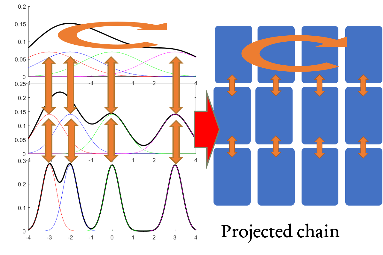
Thus the simulated tempering chain for \(\wt p_i\) mixes in time \(O(L^2D^2)\).
Simulated tempering mixes for \(p\)
But we need mixing for simulated tempering where the temperature is outside the sum, \[ p_i \propto \pa{\sumo jm w_j \exp\pa{-\fc{\ve{x-\mu_j}^2}2}}^{\be_i}. \] This follows from mixing for \(\wt p_i\), plus the fact that the ratio $ p_i/p_i$ is bounded: \(\fc{p_i}{\wt p_i}\in [w_{\min}, \rc{w_{\min}}]\). We lose a factor of \(\rc{w_{\min}^2}\). This finishes the proof of the main result.
Takeaways
- “Beyond log-concavity” for sampling is the analogue of “beyond convexity” for optimization.
- There is a spectral decomposition lemma for Markov chains based on decomposing the Markov chain rather than just the state space, and that helps prove mixing for simulated tempering.
- Provable sampling holds for a prototypical multimodal distribution: mixture of Gaussians.
Further directions
Here are further directions and open questions we would like to explore. Feel free to get in touch if you have ideas!
- How do we deal with gaussians with different variance?
- You might have wondered why we needed the gaussians to have the same covariance, and how robust the results are to different covariances. We can allow the variances to be at most a factor of \(1+\fc Cd\) apart in each direction. In general different variances have the problem that they change the mixture coefficients at the different levels - for a skinny gaussian, it could be exponentially small at the highest temperature, and large at the lowest temperature. Thus it’s hard to even get into the “attractor region” for that gaussian at the highest temperature - like finding a needle in a haystack. One assumption we can use to get around this is to assume we’re given points near each of the modes. Then we can hope to have an unbiased sample by combining the samples starting from each of those modes, with the right coefficients.
- Find practical algorithms for testing whether a Markov chain has mixed.
- Carry out average-case analysis for distributions of interest.
In real-life, the distributions we want to sample from are not as simple as a polynomial mixture of gaussians. For example, consider clustering. Suppose a simple model, that there are m clusters, each has some mean \(\mu_j\), and each point is equally likely to be drawn from each cluster. Then the posterior distribution looks like a product of sums \(\prod_{n=1}^N \pa{\sumo jm \rc m \exp\pa{-\fc{\ve{x_n-\mu_j}^2}2}}\), which when expanded out, has exponentially many terms, so our results don’t immediately apply.
One obstacle is that in many distributions \(p\) of interest, \(p\propto e^{-f}\) is not mixture of the probability distribution, but rather, \(f\) is a combination of simpler functions. In other words, \(p\propto e^{-\sum_j w_jf_j}\) rather than \(p\propto \sum_j w_j e^{-f_j}\). When this combination happens in the exponent, the decomposition approach doesn’t work so well.7
Can we come up with provable results for Ising models, stochastic/censored block models, or RBM’s?
It would be great to find other uses for our simulated tempering decomposition theorem - in principle the theorem could even apply when there are exponentially many modes, as long as we create a refining partition such that there is no “bottleneck” at any point.8
- What are the guarantees for other temperature heuristics used in practice, such as particle filters, annealed importance sampling, and parallel tempering? One undesirable property of simulated tempering is that it incurs a factor of \(O(L^2)\) in the running time, where \(L\) is the number of levels. Particle filters and annealed importance sampling move only from higher to lower temperature, and so only incur a factor of \(O(L)\). The analysis would be different because they are no longer Markov chains on \([L]\times \Om\), but similar decomposition theorems may hold.
Thoughts, questions, typos? Leave a comment below.
For example, consider when \(p(x)\) has peaks around the points of the boolean cube that satisfy a SAT formula; this is #P-hard to sample from.↩
The difference between their work and our work is that we care about about actual mixing time, rather than just hitting time for certain sets. By itself Langevin diffusion does not work well with deep, separated local minima.↩
The reason for the square-root scaling is that noise from Brownian motion scales as the square root of the time elapsed (the standard deviation of a sum of \(n\) iid random variables scales as \(\sqrt{n}\)).↩
Changing the temperature is just changing the scaling of the gradient step with respect to the noise.↩
This definition is stated for continuous Markov chains. By rate \(\lambda\) I mean that the time between swaps is an exponential distribution with decay \(\lambda\) (in other words, the times of the swaps forms a Poisson process). A version for discrete Markov chains is to swap with probability \(\lambda\) and to follow the current chain with probability \(1-\lambda\). Note that simulated tempering is traditionally defined for discrete Markov chains, but we will need the continuous version for our proof.↩
They proceed by first bounding the spectral gap for parallel tempering, and then showing the gap for simulated tempering is lower-bounded in terms of that. However, in our experience, bounding the spectral gap for simulated tempering directly is easier!↩
Think of the downstairs combination as an OR combination, the upstairs one as a AND.↩
We stated it in the case where we had the same partition at every level. The more general form of the theorem works even if the partitions on different. The bound could be polynomial even if there are exponentially many components.↩